Today’s Large Language Models (LLM) are based on Transformers, a deep learning model architecture for sequence-to-sequence transformations based on the attention mechanism. While it was originally proposed and used in Natural Language Processing (NLP) tasks like language translation, it turns out that a lot of things that we care about can be modelled in terms of sequences, making transformers a useful model in a wide variety of applications beyond NLP such as image processing and reinforcement learning . Given the overwhelming success of transformers in deep learning, I thought I should finally take some time to read and understand the paper “Attention Is All You Need” (Vaswani et al., 2017) that first proposed the Transformer architecture.

This paper is now almost 6 years(!) old. In a field as fast-moving as machine learning, one might be tempted view it as an artifact of the past, but Transformers are more relevant today than ever: LLMs that have garnered hype recently, such as OpenAI’s ChatGPT & GPT-4 as well as Google’s PaLM, are all some variants of Transformers, except trained with massive scale, both in terms of model size and training data. ¹

Given the age of this architecture, by now there are already several tutorials covering transformers online, so this article is mostly for my own learning – I find that teaching others is a really good way to understand the material deeply. If anyone else stumbles across this post and finds it helpful, that’s an added bonus 😊.

How to use this article

This article is my attempt to document – as thorougly as possible – the technical details of Transformers and how they are trained, so I can refer back to it when I forget. I wrote this piece with a more technically inclined reader in mind – someone who has had some experience with programming and perhaps even a passing interest in Artificial Intelligence but isn’t deeply involved in the field. In particular I assume you know about tensors , linear algebra and the basic components of modern deep learning, such as backprop, softmax and ReLU. And while I try to make an effort to explain the core concepts as intuitively as possible, this isn’t intended to be quick byte-sized primer on Transformers: my goal here is thoroughness in detail.

In my opinion, the core idea behind Transformers – attention – isn’t that hard to grasp. That said, I’ve found that actually getting your hands dirty and implementing the model in code can be a different story – even after understanding at a conceptual level, I ran into many practical issues trying to make training work. It is rewarding though, and you learn a whole lot, so I recommend others try too.

Table of Contents

• All about transformations
  • Overview of the Transformer architecture
  • Preprocessing
    • Step 1: Tokenization
    • Step 2: Converting tokens to vocabulary indices
  • Diving deeper into transformers
    • Step 3: Embedding
    • Step 4: Adding Positional Encoding
  • Encoder
    • Attention is all you need
    • A closer look at attention
    • Matrix formulation of attention
    • Back to Positional Encodings
    • Multi-Head Attention
    • Masking in the encoder
    • Feed-Forward Network
    • Encoder: the remaining bits
  • Decoder
    • Difference #1: Cross-Attention
    • Difference #2: Masking in self-attention
  • Linear + Softmax Layer
• Training
  • Loss function
  • Regularization
  • Model hyperparameters
  • Optimizer
  • Learning-rate scheduling
• Inference
• Conclusion
• Acknowledgements
• Where to go from here

All about transformations

At a high level, a Transformer – as its name suggests – transforms an input sequence $X=(x_1,x_2,…,x_S)$ into an output sequence $Y=(y_1,y_2,…,y_T)$. Because this formulation is so general, it doesn’t say what $x_i$ and $y_i$ should represent – it could be a word, a sub-word, a character, a pixel, or a token representing some arbitrary thing, making the Transformer architecture very versatile in a wide range of tasks. For the rest of the article, I’ll be talking about Transformers in the context of Natural Langauge Processing (NLP) tasks, because that’s what it was originally invented for. In the context of machine translation, the input sequence could be a sequence of words in one language like English, and the output could be a sequence of words in the another, like German²:

Okay, so it’s actually a bit more nuanced than that: a Transformer transforms an input sequence into an output sequence, but it does so by learning to transform an output sequence $(y_1,y_2,…,y_T)$ into another sequence $(z_1,z_2,…,z_T)$, of the same length T. This is because during training, we teach a Transformer model to predict the next element for each element in the sequence.

Suppose we want to train a Transformer model to translate English to German. Say we have an English sentence "The weather is great today" which in German would be "Das Wetter ist heute großartig". A sentence is a sequence – it can be sequence of characters, sub-words, words or even bytes, depending on how you split it up. If we split by words, we get an input sequence [The, weather, is, great, today] and a target output sequence of [Das, Wetter, ist, heute, großartig]. During training, a Transformer takes these two sequences and learns to output the sequence [Wetter, ist, heute, großartig, <eos>], where <eos> is a special token indicating that this is the end-of-sentence. Notice that its goal is to predict the German word that comes next at each position: Wetter came after Das in our original German sentence so by the end of the training, our Transformer model should spit out Wetter when its two inputs are Das and [The, weather, is, great, today]. For each pair of English-German sentences, we score the model on how well it did in its predictions, and use this to update the model’s parameters so that we get a better prediction in the next pair.

In other words, it learns to predict what word/token has the highest probability of being in position $i+1$ given A) the entire sequence sequence $Y$ up to position $i$ and B) a different sequence $X$ (in our example this was the English sentence). So really, you can think of training the model as finding a really big function $f(X,Y)$ that takes any two sequences $X=(x_1,x_2,…,x_S)$ and $Y=(y_1,y_2,…,y_T)$ and giving us a sequence $Z=(z_1,z_2,…,z_T)$ where $z_i=y_{i+1}$ at all positions except the last, and where the last element $z_T$ should be a special <eos> token to indicate the end of sentence. And remember, in a typical dataset, we might have millions of pairs of $X$ and $Y$, so this function $f(X,Y)$ has to be sufficiently large and complex to even apprximately map the inputs to the correct outputs, across all the training examples.

The magic of LLMs – still mostly Transformer-based – is that at a large enough scale (we’re talking about things like the amount of data, training compute and model size here), emergent properties, such as the ability to do complex reasoning with multiple steps, start to appear in these models.³ Somehow, by simply learning to predict the next token across a vast number of texts, these models seem to learn to represent facts about our world in their weights. I think that’s pretty neat.

Overview of the Transformer architecture

Now let’s talk about what a Transformer actually looks like. Here’s a diagram from the original paper “Attention Is All You Need” (Vaswani et al., 2017) :

If you’re like me, this might be a bit overwhelming to take in at first. In reality, there’s only 4 major components to a transformer architecture: the embedding layer, the encoder, the decoder, and the final linear+softmax layers that transform the output of the decoder into probabilities. Here’s the same diagram with some annotations overlaid on top:

Preprocessing

Let’s start from the very beginning. The original Transformer in the 2017 paper was trained on the task of translating English sentences to German, using the WMT 2014 English-German dataset. This dataset contains ~4.5 million pairs of English sentences and their corresponding translations in German, so I’ll use this example to explain what happens in a Transformer for the rest of the article.

You first need to preprocess these sentence pairs into a format that computers can understand. We do this in 2 steps:

Step 1: Tokenization

The first step is tokenization, which turns a sentence into a sequence. To be clear, this step happens outside of the transformer In this step, we transform each sentence into a sequence of tokens. During training, the input to the Transformer encoder is thus sequence(s) of tokens generated from the English sentences. The paper mentions that they used byte-pair encoding (see page 7) for tokenization, but for simplicity I’ll assume that the sentences are tokenized word by word.

Above is an illustration of what this would look like for an example mini-batch of 3 English sentences. Note that we have introduced 3 special tokens:

• <bos> denoting the beginning of sentence, which will be useful during model inference .
• <eos> marking the end of a sentence
• <pad> representing an “empty” token to make all the sequences in the tensor of the same length (i.e. the maximum sequence length across all sentences in the mini-batch) for parallel processing.

Step 2: Converting tokens to vocabulary indices

Now we have sequence(s) of English words. But English isn’t a language that computers can understand. Computers deal with numbers, so we need to first preprocess this data into a machine-friendly format before we can make those GPUs go brrr. To do this, we create a vocabulary of all the possible tokens that appear in our dataset. Then, we replace each token with its index in this vocabulary. So, the word “The” might have an index of 11, which uniquely identifies that token. We also leave out some indices for the special tokens that we introduced (<bos>, <pad> and <eos>): for example, their indices might be 0, 1 and 2 respectively. After this step, this is what we have:

To be clear, these 2 steps happen outside the Transformer.

Diving deeper into transformers

After Steps 1 and 2, we have data ready to be consumed by the Transformer model. The next 2 steps happen within the Transformer, as these steps involve trainable parameters that are updated with the rest of the Transformer model parameters.

Step 3: Embedding

In this step, we use the indices in the previous step to index into a lookup-table called an embedding and transform the indices into high-dimensional vectors that we call an embedding vectors. In PyTorch, this can be implemented using the nn.Embedding() module. In the original paper, the embedding dimension is 512 (meaning the vectors we get are 512-dimensional), but this is a hyperparameter that we can tune for our model through experiments. Note that in the paper, they also multiply the embedding weights by sqrt of the embedding dimension (see page 5).

After this step, we have a tensor of shape (batch size, input sequence length, embedding dimension). For the rest of the article, I’ll use the short form B for batch size, S for the input sequence length, and D for the embedding dimension. So in our example, B=3, S=9 and D=512. After this step, we get:

Step 4: Adding Positional Encoding

So I’m going to skim over this part for now and return to it later when it’ll make more sense why we need this step, but we need to know now is that in this step, we add some tensor (of the same shape) to our embeddings from the previous step. This tensor encodes information about the relative order of each word in a sentence (or more generally speaking, each token in a sequence), since this is information that we’d like the model to make use of to generate its predictions. This will come in useful for the next section on Attention .

To recap: we started with B=3 English sentences and turned each sentence into a sequence of words and introduced special tokens representing start and end of each sentence. Then we added padding tokens to make all 3 sequences of the same length S=9. After that, we turned each token/word into its corresponding index, and used that index to retrieve an embedding vector with D=512 dimensions. As a final step, we added a special “position encoding vector” giving us a final tensor of shape (B,S,D), which is now ready to pass to our first encoder. The same process happens with the target sequence (i.e. German sentences), except we pass it to the decoder instead.

Encoder

Next we have the Transformer encoders. The encoding step consists of N independent encoder units stacked on top of each other. These encoders are identical in architecture, but do not share weights between them and are thus separately updated during backpropagation.

The encoder unit itself comprises 2 parts:

1. A Self-Attention module
2. A Feed-Forward Network

I’ll start with this high level picture of the encoder and gradually fill in more details.

Attention is all you need

The core idea behind Transformers is to replace recurrence and convolutions that made up previous sequence-to-sequence models almost entirely with the attention mechanism. In oversimplified terms, the attention mechanism is basically just taking a bunch of dot products between embeddings in our sequence. And self-attention is just particular case of attention where the sequences are actually all the same – just one sequence.

Remember that at this point, our example input is a tensor of shape (3,9,512). To make the explanation easier, let’s look at what happens for one particular sentence out of 3 in this mini-batch (i.e. let’s consider an example with batch size of 1). This can be easily extrapolated to higher batch sizes.

Let’s look at just one sentence: "This jacket is too small for me". From this, we get a tensor of shape (9,512). To encode this tensor, we first pass all 9 of the 512-dimensional embedding vector to the self-attention module at the same time:

The goal of the self-attention module is to figure out how the words in the sentence (or more generally, tokens in a sequence) relate to each other. For example, when we look at the adjective "small", we want to understand what object it is referring to. Clearly, we know that it is referring to the noun "jacket", but the Transformer model has to learn this. In other words, it has to learn how each word relates to another.

A closer look at attention

In vector space, we have a concept for computing the similarity between vectors: dot product. And dot products form the basis of the attention mechanism. I’m partly limited by my choice of medium here: I think the math looks overly dense on text, so I recommend you watch this lecture instead if you’re looking for a really good overview of transformers. I’m including these sections on attention for thoroughness’ sake.

Computing attention involves 3 inputs: query(s), keys(s), and value(s) where these are all vectors. More formally, we have:

• Queries $q_1,…,q_{N_q}$ where $q_i \in$ $\mathbb{R}^{d_k}$, where $d_k$ is the dimension of the query vector, and $N_q$ is the number of queries
• Keys $k_1,…k_{N_k}$ where $k_i \in$ $\mathbb{R}^{d_k}$, and $N_k$ is the number of key-value pairs
• Value $v_1,…,v_{N_k}$ where $v_i \in$ $\mathbb{R}^{d_v}$, where $d_v$ is the dimension of the value vector, which is not necessarily equal to $d_k$, although in our example of English-German translation, it is.

Note that $N_q$, the number of queries doesn’t necessarily have to equal $N_k$, the number of key-value pairs, but the number of keys must be the same as the number of values (for them to form a key-value pair). Furthermore, the query and key vectors must have the same dimension, $d_k$ so we can perform a dot product.

Given this formulation, the output at position $i$ is computed using the following steps:

• Get dot product of query and key vectors to get a scalar value: $\alpha_{ij} = q_i \cdot k_i$
• Normalize each dot product $\alpha_{ij}$ by performing softmax across all $j$, where $j=1,…,N_{k}$ , where $N_{k}$ is the number of key-value pairs. This gives us weights $w_{ij}$ for all $j$.
• The output at position $i$ is the weighted sum of all $v_j$ where weight of $v_j$ is $w_{ij}$.

Back to our example sentence, we have $x_1,…,x_9$ where $x_i$ is a 512-dimensional embedding vector representing each word in the sentence "This jacket is too small for me" plus the <bos> and <eos> tokens. We obtain our query, key and value vectors from $x_i$ by multiplying it each time with a different matrix:

In our case, $d_k=d_v=512$. We have $W^K$, $W^Q$ and $W^Q$ matrices that linearly project each key, query and value vectors – this allows for more flexibility in both how the model chooses to define “similarity” between words (by updating $K$ and $Q$), as well as what the final weighted sum represents (by updating $V$) in latent space. Remember, the values in these weight matrices are being updated over the course of the training via backprop. In Pytorch code, these matrices are implemented as nn.Linear modules with bias=False.

Now that we have $k_i$, $q_i$ and $v_i$, we just compute the corresponding output for $x_i$ using the steps outlined earlier, computing the sum of all vectors weighed by the dot products. Here, since $q_i$, $k_i$ and $v_i$ are all derived from $x_i$, we give it a special name: self-attention.

Matrix formulation of attention

As you can see, attention is computed using dot products between any two words within a sequence, allowing the Transformer to learn long-range dependencies in a sequence more easily. One downside of this, though, is that the computation of attention scores is quadratic in the length of the input sequence $N$. This quadratic $O(N^2)$ complexity is an issue because it means it will take a lot of compute for long sequences.

On the upside, we can represent the computation as a product of a few matrix multiplications, which is easily parallelizable on GPU/TPUs. Given row-major matrices $Q$, $K$ and $V$ containing rows of query, key and value vectors respectively, the general formulation of attention in matrix form is as follows:

\begin{equation} Attention(Q,K,V) = softmax(QK^T)V \end{equation}

Again, the $Q$, $K$ and $V$ matrices are computed using the corresponding weight matrices $W^Q$, $W^K$, and $W^V$: for example, if we have a matrix $A$ where each row is an embedding vector in our sequence, then we’d have $Q=AW^Q$, $K=AW^K$ and $V=AW^V$ for the self-attention sublayer in the encoder. As we’ll see later when we get to cross-attention in the decoder, $Q$, $K$ and $V$ do not necessarily need to come from a single matrix $A$.

The authors in the Transformers paper also apply a scaling factor of $\frac{1}{\sqrt{d_k}}$ to the matrix of dot products (numerator) to prevent the products from becoming too large, which can “[push] the softmax function into regions where it has extremely small gradients” (Viswani et al, 2017, page 4 ):

\begin{equation} Attention(Q,K,V) = softmax(\frac{QK^T}{\sqrt{d_k}})V \end{equation}

This ability for parallelization is an important reason why Transformers have been so successful – previous models based on recurrence, for example, cannot be parallelized because the computation of its state $h_t$ at time $t$ necessarily depends on the computation of its previous state $h_{t-1}$ at time $t-1$.

Another important consequence of relying heavily on attention is that we can easiljy visualize the attention weights, which can aid in debugging as well as interpreting and explaining the model output.

Back to Positional Encodings

Finally, we can finally talk about why we need positional encodings , which we skimmed over earlier. We’ve seen that attention basically comes down to taking a bunch of dot products and taking a weighted sum. The problem is, by simply taking dot products, we lose information about the relative order of these words in a sentence. And intuitively, we know that the position of a word in a sentence matters.

To encode information about the position of each token in the sequence, we add positional encodings to the input embeddings (refer back to Step 4 of our embedding stage). In practice, there are many ways to generate this – including having the network learn this during training – but the authors generate static encodings using following formula:

$$ \begin{aligned} PE_{(pos,2i)} &= \sin(pos/10000^{2i/d_{emb}}) \\ PE_{(pos,2i+1)} &= \cos(pos/10000^{2i/d_{emb}}) \end{aligned} $$

where $i$ is the index along the embedding dimension and $pos$ is the position of the token in the sequence. Both are 0-indexed. By having sine and cosine functions of varying periods, we are able to inject information about position in continuous form. Remember, these are static values and not updated during training. I included the formula for completeness but really, the easiest way to understand is by visualising it with a graph:

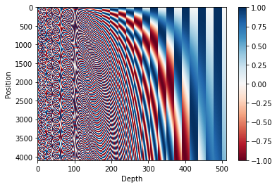
I don’t have much else to add on positional encodings, though I’ll point out that the periodic nature of sinusoids used here has some nice properties, like placing more emphasis on relative – as opposed to absolute – order (see Stanford CS224N Lecture 9 - Self-Attention and Transformers )

class PositionalEncoding(nn.Module):
  def __init__(self, emb_dim: int, max_seq_len: int = 5000):
    super().__init__()
    assert emb_dim % 2 == 0, "Embedding dimension must be divisble by 2"
    self.dropout = nn.Dropout(0.1)
    
    pos = torch.arange(max_seq_len)[:, None] # [seq_len, 1]
    evens = 10000. ** (-torch.arange(0,emb_dim,step=2) / emb_dim)
    evens = evens[None, :] # [1, ceil(emb_dim/2)]
    evens = pos * evens # [seq_len, ceil(emb_dim/2)]
    pe = rearrange([evens.sin(), evens.clone().cos()], 't h w -> h (w t)') # interleave even and odd parts
      
    self.register_buffer('pe', pe) # [max_seq_len, emb_dim]
  
  def forward(self, 
              src: Tensor # [bsz, seq_len, emb_dim]
              ) -> Tensor:
    assert src.shape[-1] == self.pe.shape[1], f"Expected embedding dimension of {self.pe[1]} but got {src.shape[-1]} instead."
    out = src + self.pe[None,:src.size(1),:]
    return self.dropout(out) # apply dropout

Multi-Head Attention

We’re not done with attention yet. So far, I’ve talked about self-attention with just one so-called “head”. In the paper, the authors use Multi-Head Attention (MHA). In MHA, we have multiple heads that each performs the attention computation independently. Each head $\textbf{head}_i$ has its own linear projection matrices $Q_i$, $K_i$, and $V_i$, and these matrices project the query, key and value vectors to a lower dimensional space than we had with single matrices.

For example, if the dimension of matrix $K$ in Single-Head Attention was $512 \times 512$, then the dimension of $K_1$ and $K_2$ in a 2-Head Attention would each be $512 \times 256$, thus projecting to a 256-dimensional space instead of 512-dimensional. After all the heads compute its own value of $\text{Attention}(Q_i,K_i,V_i)$ in parallel, we concatenate the outputs to obtain an output of the same shape (256+256=512) as we had in the case of single-head attention.

Unlike for single-headed attention, we also have an additional step: a linear projection to $d_{emb}$-dimensional space again using matrix $W_i^O$ where $d_{emb}$ is the embedding dimension. For an input of shape (B,S,D), MHA thus produces an output of the same shape.

The intuition behind why having multiple heads improves performance is that by having independently trainable linear projections per head, the model is able to simultaneously attend to different aspects of the language (for example, for a model trained on LaTeX documents, it might have one head that learns to attend to a presence of a \end command if a \begin command appears in the sequence, and another head that relates words in terms of their semantic relevance in text).

class MultiHeadAttention(nn.Module):
  def __init__(self,
               emb_dim: int,
               n_heads: int):
    super().__init__()
    assert emb_dim % n_heads == 0, "Embedding dimension must be divisble by number of heads"
    self.n_heads = n_heads
    self.emb_dim = emb_dim
    self.head_dim = emb_dim // n_heads
    # This projects each word vector into a new vector space (and we have n_heads amount of different vector spaces)
    self.weight_query = nn.Linear(self.emb_dim, self.emb_dim, bias=False) 
    self.weight_key = nn.Linear(self.emb_dim, self.emb_dim, bias=False) 
    self.weight_value = nn.Linear(self.emb_dim, self.emb_dim, bias=False) 
    self.out_project = nn.Linear(self.emb_dim, self.emb_dim)
  
  def forward(self, 
              query: Tensor, # (B, q_seq_len, D)
              key: Tensor, # (B, kv_seq_len, D)
              value: Tensor, # (B, kv_seq_len, D)
              mask: Optional[Tensor] = None, # (B, 1, 1, kv_seq_len) or (B, 1, q_seq_len, q_seq_len] where q_seq_len == kv_seq_len for self-attention
              ) -> Tensor:
    bsz, q_seq_len, _ = query.shape

    Q = self.weight_query(query)
    K = self.weight_key(key)
    V = self.weight_value(value) 
    Q,K,V = [x.view(bsz, -1, self.n_heads, self.head_dim).transpose(1,2) for x in (Q,K,V)]

    attn_weights = torch.einsum('bhqd,bhkd->bhqk',[Q,K]) # (B, number of heads, q_seq_len, kv_seq_len] 
    attn_weights /= math.sqrt(self.head_dim) 

    if mask is not None:
      attn_weights += mask

    # softmax across last dim as it represents attention weight for each embedding vector in sequence
    softmax_attn = F.softmax(attn_weights, dim=-1) 
    out = torch.einsum('bhql,bhld->bhqd',[softmax_attn, V]) # (B, number of heads, q_seq_len, D/h]
    out = out.transpose(1,2).reshape(bsz, -1, self.n_heads * self.head_dim) # (B, q_seq_len, D)
    return self.out_project(out)

Masking in the encoder

The last important detail to mention at this point for the encoder is masking. Recall that in our input sequence, we used a special token for padding, <pad>. Because these are just dummy tokens added to ensure all sequences in a batch are of the same length, during attention computation we’d like to exclude the embedding vectors corresponding to these padding tokens from the weighted sum, by setting their weights to 0.

To do this, we can’t just set the weights in the corresponding positions to 0 after softmax, because then the weights will no longer sum to 1. Instead, we can apply a mask to the dot products before softmax such that after softmax, their values become 0. This can be achieved by adding negative infinity ($-\infty$) to positions corresponding to the padding tokens:

In PyTorch, you can create a padding mask like so:

def create_padding_mask(xs: Tensor, # (B, N)
                        pad_idx: int 
                        ) -> Tensor:
  batch_size, seq_len = xs.shape
  mask = torch.zeros(xs.shape).to(device)
  mask_indices = xs == pad_idx
  mask[mask_indices] = float('-inf')
  return mask.reshape(batch_size,1,1,seq_len) # (B, 1, 1, N)

The create_padding_mask() function takes a PyTorch tensor of shape (B,N) and the index of the padding token in vocabulary and returns a mask of shape (B,1,1,N) where B is the batch size and N is the length of the sequence passed in. There are 2 additional dimensions in the output because of the way we apply the mask in MHA (refer to the reference implementation):

attn_weights += mask

The shape of attn_weights is (B, number of heads, query_sequence_len, key_value_sequence_len) where h is the number of heads. Since mask has shape (B,1,1,key_value_sequence_len), we broadcast across the 2nd and 3rd dimensions. While query_sequence_len equals key_value_sequence_len in self-attention, this will no longer necessarily be true when we look at cross-attention in the decoder. This is why we don’t generate a padding mask of shape (B,1,N,N), although we technically can for self-attention.

Feed-Forward Network

Recall that self-attention is only the first part of a Transformer encoder. The issue with only having self-attention is that it is a linear transformation with respect to each element/position in a sequence; as we have seen, self-attention is basically a weighted sum (linear) where the weights are computed from dot products (also linear). And we know that nonlinearities are important in deep learning because it allows neural networks to approximate a wide range of functions (or all continous functions, as the Universal approximation theorem tells us).

So the creators of the Transformer introduce a fully connected feed-forward network (FFN) after attention. The FFN is applied position-wise, meaning it is applied to each element in the sequence independently. Therefore, in addition to introducing nonlinearities, these FFNs can also be thought of as somehow “processing” the individual outputs in the sequence post-attention – it does this by projecting the input into a higher dimension, applying nonlinearity, and projecting it back into the original dimension.⁴ In the paper, they use a 2-layer network with 1 hidden layer and ReLU activation as the nonlinearity. In PyTorch, this simply implemented as:

feed_foward_net = nn.Sequential(
    nn.Linear(embedding_dimension, hidden_dimension),
    nn.ReLU(),
    nn.Linear(hidden_dimension, embedding_dimension),
) 

In the paper, hidden_dimension is set to a value of 2048 (embedding_dimension is 512 as mentioned earlier).

To recap: if we have a tensor of shape (9,512) at the start of the encoder, after passing through Multi-Head Attention, we get back an output of the same shape. When we pass this through the FFN as defined above, we basically pass each of the nine 512-dimensional vectors through the neural network in parallel and join them together to get back a final output tensor of the same shape (9,512). This works because the last dimension of the input tensor (512) is the same as the dimension of the input features of the FFN. The same analysis holds for higher batch sizes.

Encoder: the remaining bits

Here are the remaining details for the encoder:

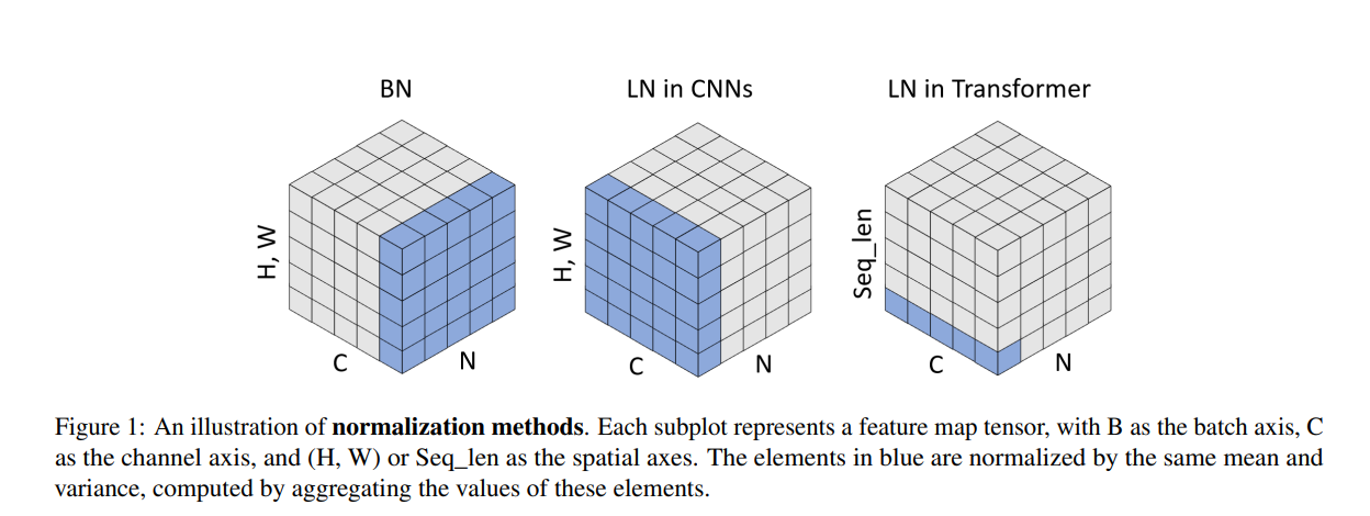
• Layer normalization is applied to the output of each sublayer. Personally, I was confused by this initially because some illustrations of how layer norm works uses layer norm in the context of Computer Vision and Convolutional Neural Networks, which is slightly different from how it is used in Transformers (be careful, some explanations online confuse between the two as well). For this, I’ve found the following figure from the paper “Leveraging Batch Normalization for Vision Transformers” (Yao, Zhuliang, et al., 2021) to be helpful in visualising the key difference between layer norm in CNN and in transformers:

• Use of residual connections around both the self-attention and feed-forward network sublayers. First introduced in 2015 by the famous ResNet paper , residual connections here basically means instead of the sublayer output being f(x), it is x + f(x), which helps with training by providing a gateway for gradients to pass through more easily during backprop.

Let’s end this section by revisiting the encoder diagram from the paper:

Everything shown in the diagram should be familiar to us by now. In particular, note how there are 3 arrows going into the Multi-Head Attention module: these represent the queries, keys and values.

Decoder

Phew! There was quite a lot to cover for encoders. Fortunately, I’ve already covered most of the important parts of the Transformer – the decoding part is similar what we had in the encoding phase, with a few key differences.

Similar to the encoders, the input to the first decoder is the embeddings (+positional encodings) of the target sequence. In the context of English-to-German translation, the target sequence would be German sentences in our training dataset. These are transformed into embeddings through the process outlined earlier .

Also similar to the encoding phase, we have $N$ decoder modules, where $N=6$ for the base model in the original paper. Each decoder is similar to the encoder, except there are 2 differences:

• In a decoder, there is an additional sublayer between self-attention and feed-forward network: cross-attention.
• An additional mask is used in the decoder to prevent “looking into the future” in self-attention.

Difference #1: Cross-Attention

Remember that in self-attention, we derive the query, key and value vectors from the same embedding vector. In cross-attention, we derive the query vector from one embedding vector and key and value vectors from a different vector. More specifically, in the decoder, the query vector comes from the output of the previous layer (i.e. for the very first decoder, this is the embedding layer; for subsequent decoders, it’s the previous decoder), while the key and value vectors are generated from the output of the last encoder. Referring back to Figure 1 from the paper, this is illustrated with two arrows coming from the encoder to the cross-attention sublayer of the decoder.

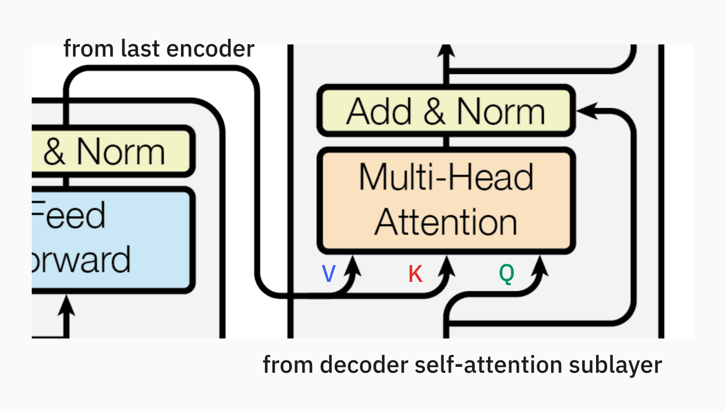
Again, in the context of machine translation, this makes intuitive sense because for each word in the target language sentence, we are basically querying for the most relevant word(s) in the source language sentence and taking a weighted sum of their vector representations in order to predict the next word.

Masking in cross-attention Let’s wrap this part up by talking about masking in cross-attention. In cross-attention, because the key and value vectors that we’re using to calculate dot products and calculate the weighted sum respectively come from the final output of the encoder, we don’t need to mask future tokens, because all of the information about the source sequence $X$ should be available to us in the decoding stage. For example, when we are doing machine translation, we have available to us a sentence in the source language – this information should be fully available to the model during training. However, we still need to mask out the positions which correspond to padding tokens in the encoder’s input like we did for self-attention in the encoder.

Recall the shape of the padding mask , which was (B,1,1,S), where S is the length of the source token sequence. Let’s think about the shape of the dot product matrix, $QK^T$. $QK^T$ is a matrix $\in \mathbb{R}^{T \times S}$, where T is the target token sequence length. When we consider multiple heads and batch size, then the result of our attention weights will be of shape (B,number of attention heads,T,S). So PyTorch broadcasts across the 2nd and 3rd dimensions again when we add the padding mask.

Difference #2: Masking in self-attention

The other difference between decoders and encoders is in the masks used in self-attention.

Unlike in the encoder, the decoder shouldn’t access information about future positions to make a prediction for any given position in the sequence – otherwise, the prediction would be trivial and the model won’t learn. Therefore, we apply a mask to exclude future positions from the weighted sum calculation in self-attention. Again, this is achieved by setting these weights to $-\infty$ befre applying softmax.

As you can see, this mask has $-\infty$ in the upper triangular part. I don’t think there’s an official name for this mask, so I’ll call it the look-ahead mask. Here’s the PyTorch code that generates this mask:

def create_decoder_mask(seq_len: int) -> Tensor:
  mask = torch.zeros(seq_len, seq_len).to(device)
  mask_indices = torch.arange(seq_len)[None, :] > torch.arange(seq_len)[:, None] 
  mask[mask_indices] = float('-inf')  
  return mask.reshape(1,1,seq_len,seq_len) # (1, 1, N, N)

The function takes in the length of the target sequence and returns a mask with shape (1,1,N,N) where $N$ is the sequence length. Recall that the self-attention mask for the encoder had shape (B,1,1,N). In the decoder, I’ve set the first dimension as 1 for broadcasting, but it can very well be B as well. However, the third dimension has to be N and not 1, since the mask used in the decoder is two-dimensional, and thus needed to be $N \times N$.

Linear + Softmax Layer

As a final step, the output from the last decoder is passed to a linear layer that projects the embedding vectors to a dimension given by the vocabulary size of the target language (you can also have a shared vocabulary between source and target languages), followed by a softmax layer to convert those values into probabilities that sum to 1.

For example, if we translating from English to German, and the dataset we’re training on has a German vocabulary size of 37000, then the linear layer will take emb_dimension input features (e.g. 512) and have 37000 output features. After softmax, the value at $i^{th}$ dimension of the vector at $k^{th}$ position in the sequence is the probability for the $i^{th}$ word/token in the vocabulary to appear in the $(k+1)^{th}$ position.

Training

Now let’s talk about training. Again I’ll talk about training in the context of machine translation.

In a typical training dataset, like the WMT 2014 English-German dataset, you’ll have pairs of (sentence in source langauge, same sentence in target language). As mentioned earlier , you’ll first need to preprocess the text. Then, during training, the Transformer is scored on how well it can predict the next token for each position. In code, you’d do something like:

target_input = target[:,:-1]  # shifted one to the right
target_predict = target[:,1:] # shifted one to the left

where target_input is an input to the model – this is the input sequence $Y$ we’ve been talking about – and is shifted one to the right, and the model is scored on how close its outputs are to target_predict, which is the target output sequence $Z$ obtained from shifting the original target sequence one to the left.

To give a concrete example:

• The source sequence is [<bos>, The, man, is, happy, <eos>, <pad>, <pad>]
• The translated target sequence in German is [<bos>, Der, Mann, ist, glücklich, <eos>, <pad>, <pad>]
• The input to the encoder is the embeddings of [<bos>, The, man, is, happy, <eos>, <pad>, <pad>], the original source sequence.
• The input to the decoder is the embeddings of [<bos>, Der, Mann, ist, glücklich, <eos>, <pad>] (shifted one right)
• The decoder should predict [Der, Mann, ist, glücklich, <eos>, <pad>, <pad>] (shifted one left)

Loss function

The paper doesn’t explicilty mention what loss function is used, but you should be able to use any multi-class classification loss (which is what we’re doing when predicting the most probable next token). The implementations I’ve seen online use either cross-entropy or KL divergence loss. In my own implementation, I used cross-entropy loss.

A mistake that cost me a lot of time debugging was how nn.CrossEntropyLoss works in PyTorch. In PyTorch, this module performs softmax before calculating the actual cross entropy loss – it should really be named something like nn.SoftmaxCrossEntropyLoss! Because the figure of the Transformer architecture in the original paper has a softmax layer, this is what I originally implemented, and I was passing these normalized logits directly to nn.CrossEntropyLoss, causing issues during training: loss plateauing and my model quickly converging to producing the same tokens. In fairness, the PyTorch docs does mention that it expects an input that “contains the unnormalized logits for each class (which do not need to be positive or sum to 1, in general)” but who has time to read documentation, am I right? 😏

When calculating the loss, it’s important to ignore the loss contributed by the positions that correspond to the padding tokens. Referring to the look-ahead mask in the decoder, the mask prevents the embeddings of padding tokens from being included in the weighted sum in attention in non-padding positions, but we nevertheless still compute the weighted sum for the padding positions. If this was the final output of the last decoder, after passing through the linear layer and thereafter taking softmax, we would have the next-token probabilities at each position, even where we had paddings! So we’d like to exclude these positions from our loss, since we don’t really care about padding tokens anyway. In nn.CrossEntropyLoss, you can do this by passing the index of <pad> to the ignore_index argument:

criterion = nn.CrossEntropyLoss(ignore_index=PAD_IDX, label_smoothing=0.1)

This loss also specifies a 10% label smoothing regularization – let’s talk about that next.

Regularization

Section 5.4 of the “Attention is all you need” paper mentions two regularization techniques used during training:

1. Label smoothing of 10% is also used in the loss calculation. The idea is simple: instead of the target distribution being one-hot (i.e. the “target” word has probability 1 and the rest of the words have 0), we set the probability of one word to be 0.9 and then distribute the other 0.1 over rest of the words in the vocabulary. This gives the model more flexibility in what token it predicts and presumably improves training. Intuitively, this kind of smoothing makes sense because with languages, there are often many plausible words that can come after some sequence of them.
2. Dropout is used after each sublayer in the encoders, decoders, as well as to all the embeddings. The authors used a 10% dropout for the base model.

Model hyperparameters

Model hyperparameters for the base Transformer model can be found on Table 3 of the paper. This model has around 65M trainable parameters – comparing this number to the number of trainable params in your own implementation is a helpful sanity check to perform during development.

Optimizer

Nothing special here, just an Adam optimizer with $\beta_1=0.9$, $\beta_2=0.98$ and $\epsilon=10^{-9}$.

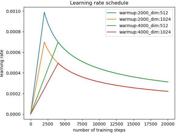
Learning-rate scheduling

The paper uses a variable learning rate during training, given by the following formula:

\begin{equation} lrate = {d_{model}}^{-0.5} \cdot min(step\texttt{_}num^{-0.5}, step\texttt{_}num \cdot warmup\texttt{_}steps^{-1.5}) \end{equation}

where $warmup\texttt{_}steps=4000$.

The best way to understand how this works is to look at how the learning rate changes with step count:

If you got the model and training steps right, you should be seeing a sweet training loss curve like this (I trained my model on translating German to English):

…and it’s learning!

Inference

Now, let’s talk about how the Transformer works at inference time for machine translation. Transformers are auto-regressive, meaning that they predict a next token from all the previous tokens. At inference time, the only data available to us is the sentence(s) in the source language. From this, how do we generate the translated text using our trained model?

This is achieved by using the <bos> token we introduced earlier to kickstart the predictions. In the beginning, our target input sequence $Y$ just contains the embedding of the <bos> token, while our source sequence $X$ are the embeddings of the English sentence. To recap , Transformers can be thought of as a function $f(X,Y)$.

1. Pass $X$ and $Y$ (initially just containing <bos>) to the trained model. From the output of the model we get a probability distribution over the vocabulary of the target language.
2. Choose the token with the highest probability and append this token to $Y$, giving us a longer sequence.

All we have to do now is to simply repeat steps 1 and 2 until the last predicted token is <eos>, marking the end of sentence. Viola! We just translated from one language to another.

Note that we still have to use the padding and the look-ahead masks just like we did for training, and with each iteration we would have to use a different look-ahead mask with each iteration since the target sequence length $T$ changes. However, more advanced implementations of Transformer can allow only the last predicted token to be passed in on each iteration , in which case the look-ahead mask doesn’t have to be passed in, since there is no “future” to consider.

Conclusion

So there it is – a thorough walkthrough of the Transformer architecture. I mostly drew examples from English-to-German language translation task, but the generality of the architecture means that this can be adapted for any sequence-to-sequence transformations, such as but not limited to summarization, code generation and Q&A.

As I mentioned in the beginning of this article, I wrote this post mostly for myself as a sort of recap of what I’ve learned, so there might be some rough edges here and there. I’m still hopeful this article might be of value to anyone who stumbles across it, especially if they are somewhat new to deep learning: most tutorials I’ve seen tend to gloss over some details around masking as well as how the textual data gets preprocessed and turned to key, query and value vectors for attention.

On a broader reflection, I find it fascinating that this same base architecture when scaled up can get us most of the way to seemingly intelligent machines capable of performing a wide range of tasks. However, I’m left feeling dissatisfied with my (and likely, our collective) understanding of why LLMs works so well and how something remotely close to what we might call intelligence can arise from performing a bunch of matrix products, so that’s an avenue of research I’m hoping to explore next.

Acknowledgements

Here are some resources that I’ve used to learn about Transformers

• Stanford CS224N Lecture 9 - Self-Attention and Transformers . Probably the best lecture on Transformers online. This is the video that made attention and Transformers click for me.
• PyTorch implementation of Transformer by Gordic Aleksa (AI Epiphany) and the accompanying video tutorial . I didn’t refer to the implementation for the most part, but I did use it as reference to debug an issue I had with my implementation.

I’d also like to thank my friend Filippo for his feedback.

Where to go from here

As an addendum, I’ll just include some links to resources that I’ve come across that might serve as good next steps after understanding the Transformer. These are also things I’d like to read up in the near future:

• A review of Transformer family of models
• Mechanistic Interpretability research
  • Related: A Mathematical Framework for Transformer Circuits
• Kaparthy’s GPT from scratch
• GPT in 160 lines of numpy
  • Related: check out my previous blog post on CNNs from scratch in numpy .
• BERT: Pre-training of Deep Bidirectional Transformers for Language Understanding
• Linformer: Self-Attention with Linear Complexity
• Flash Attention