Convolutional Neural Networks from Scratch

In this blog post we are going to take a look at how to implement a simple CNN model from scratch in Python, using mostly just numpy.

In practice, we can use high-level libraries such as Keras or PyTorch to abstract away the underlying details of CNN when writing code. However, we find that the exercise of writing one from scratch is very helpful in gaining a deeper understanding of CNNs and how these frameworks work under the hood.

Let’s get started!

Convolutions

We won’t have a CNN without some convolutional layers! Let’s start by implementing a convolutional layer class. All layers that we are going to implement in this post will be defined by a simple interface: all of them will have a forward and backward method for the forward and backward pass respectively.

This will be easier to explain once we have some code to refer to. So here it is:

import numpy as np

class Conv:
  def __init__(self, in_channels, out_channels, filter_size, pad = 0, stride = 1, weight_scale = 1e-3):
    self.pad = pad
    self.stride = stride
    # Weights initialized from 0-centered Gaussian with standard deviation
    # equal to `weight_scale` (by default set to 1e-3) for stability
    self.filters =  np.random.randn(out_channels, in_channels, 
                                     filter_size, filter_size) * weight_scale
    # biases initialized to zero
    self.bias = np.zeros((out_channels, ))


  def calc_output_dim(self, x):
    _, H, W = x.shape
    _, _, filter_height, filter_width = self.filters.shape

    H_out = 1 + (H + 2 * self.pad - filter_height) // self.stride
    W_out = 1 + (W + 2 * self.pad - filter_width) // self.stride

    return H_out, W_out


  def iterate_regions(self, x):
    H_out, W_out = self.calc_output_dim(x)
    F, C, filter_height, filter_width = self.filters.shape

    for i in range(H_out):
      for j in range(W_out):
        x_region = x[:, i * self.stride : i * self.stride + filter_height, j * self.stride : j * self.stride + filter_width]
        yield i, j, x_region


  def forward(self, x):
    """
    Inputs:
    - x: An ndarray containing input data, of shape (C, H, W)
    Returns:
    - out: Result of convolution, of shape (F, H', W') 
    where F is the number of out channels and 
    H' = 1 + (H + 2 * pad - filter_height) / stride
    W' = 1 + (W + 2 * pad - filter_width) / stride
    """

    self.x = x  # save as cache

    _, H, W = x.shape
    F, _, _, _ = self.filters.shape

    # to pad last two dimensions of the four dimensional tensor
    x_pad = np.pad(x, self.pad, mode='constant')

    H_out, W_out = self.calc_output_dim(x)
    out = np.zeros((F, H_out, W_out))

    for f in range(F):
      # convolve F times to get F x filter_height x filter_width 
      kernel = self.filters[f] # dimension is C x filter_height x filter_width    
      for i, j, x_region in self.iterate_regions(x_pad):
        out[f, i, j] = (x_region * kernel).sum()
      
      out[f] += self.bias[f] # makes use of broadcasting

    return out


  def backward(self, dout):
    """
    Inputs:
    - dout: An ndarray of the upstream derivatives, of shape (F, H', W')
    Returns a tuple of:
    - dx: Gradient w.r.t input x, of shape (C, H, W)
    - dw: Gradient w.r.t. filters, of shape (F, C, filter_height, filter_width)
    - db: Gradient w.r.t the biases, of shape (F, )
    """

    _, H, W = self.x.shape # retrieve from cache
    F, C, HH, WW = self.filters.shape
    
    x_pad = np.pad(self.x, self.pad, mode='constant')

    dx = np.zeros_like(x_pad) 
    dw = np.zeros_like(self.filters) 
    db = np.zeros_like(self.bias)

    for f in range(F): 
      for i, j, x_region in self.iterate_regions(x_pad):
        dw[f] += dout[f, i, j] * x_region

        dx[:, i*self.stride:i*self.stride + HH, j*self.stride:j*self.stride + WW] += \
              dout[f, i, j] * self.filters[f]

      db[f] += dout[f].sum()

    # trim off padding so that dimension of dx is the same as x
    dx = dx[:, self.pad: self.pad + H, self.pad : self.pad + W]

    return dx, dw, db

Convolutional layer: forward pass

In the forward call, we pass in the input image x, which will be a numpy ndarray of dimensions C x H x W where C is the number of channels (3 for RGB) and H and W are the height and weight of the image respectively.

The first thing we do is to cache the input so that we have access to it during the backpropagation:

 self.x = x  # save as cache

Following that, we pad the image with the specified padding, using 0 as the value for the padded cells. To do this, we make use of numpy’s np.pad method:

x_pad = np.pad(x, self.pad, mode='constant')

Following this, we define out, which is the tensor / ndarray we will return from forward as the result of the convolution. This will be a three-dimensional tensor with dimensions F x H_out x W_out, where F is the number of filters we specified. We calculate H_out and W_out using a formula which we extract out to a separate helper function, calc_output_dim().

H_out, W_out = self.calc_output_dim(x)
out = np.zeros((F, H_out, W_out))

Next comes the main logic for calculating the result of the convolutional operation:

for f in range(F):
      # convolve F times to get F x filter_height x filter_width 
      kernel = self.filters[f] # dimension is C x filter_height x filter_width    
      for i, j, x_region in self.iterate_regions(x_pad):
        out[f, i, j] = (x_region * kernel).sum()

For each filter, we calculate the result of multiplying the filter (filter is a reserved keyword in Python, so we use the variable name kernel) with each region in the image of the same dimension as the filter (recall the CNN theory lecture), and set the output to be returned. Here we make use of the helper function iterate_regions(), which is a generator that yields regions of the image x_pad which are of the same dimensions as the kernel (keeping the stride into account, as well).

Convolutional layer: backward pass

In the backward pass, we pass in dout, which are the upstream gradients which are being propagated from the next layer. In particular, dout is the partial derivative of our loss function (in the context of classifying digits in MNIST with CNNs, this would be the cross-entropy loss w/ softmax) with respect to the output of forward, which is a 3-dimensional tensor of dimensions F x H_out x W_out, as we previously calculated.

Given dout and the cached input, our job is to calculate dx, dw, db, which are the partial derivatives of the loss with respect to the input, filters (w stands for weights), and the biases respectively. The dimensions of each of these will be the same as the dimensions of the variables we are taking the derivative with respect to. In backward(), we return these derivatives as a tuple. dx is used as the dout for the previous layer (recall how backpropagation works!), while dw and db will be used to update the filter weights and biases respectively via gradient descent. I’ve omitted the nitty-gritty details of how to do this here in order to keep it (relatively) concise, but the implementation should be relatively straightforward once you have these gradients.

Now let’s look at the backpropagation in greater detail:

Theory

Let’s see how we can calculate dw first. To recap, dw is the gradient of the loss w.r.t the filter weights $w$ : $\frac{\partial L}{\partial w}$.

Let the output of conv (variable out from the forward pass) be $o$. Using the chain rule, we get: $\frac{\partial L}{\partial w} = \frac{\partial L}{\partial o} * \frac{\partial o}{\partial w}$. We already know $\frac{\partial L}{\partial o}$ — this is the upstream gradient dout. Now we only need to calculate $\frac{\partial o}{\partial w}$, which is the gradient of the output w.r.t to the filter weights. Let’s think about how to calculate this.

Imagine we have a 3 x 3 image $x$ and a 2 x 2 kernel filled with zeros. The result of the convolution operation is a 2 x 2 output also filled with zeros (rightside of the arrow). We assume no padding and a stride of 1:

Now let’s imagine what would happen if we nudge the value of the top left cell of the filter, such that it becomes a 1. How would the output change? After all, this is essentially what $\frac{\partial o}{\partial w}$ is telling us. Let’s look at the updated diagram:

Can you see the pattern? We can see that the output changed by exactly the image pixel values that the changed filter weight is multiplied with during the convolution operation. In other words, the derivative of a single pixel of our output $o$ with respect to a filter weight is just the corresponding pixel value in the image (that this filter weight is multiplied by).

More formally, if we let $o$ to be $m$ x $n$ and the filter to be $w$ x $h$, then the $i^{th}$ row and $j^{th}$ column of the output $o$ (which we denote by $o[i,j]$) can be expressed as:

\begin{equation} o[i,j] = \sum_{r=0}^{w} \sum_{c=0}^{h} x[i + r, j + c] * filter[r,c] \end{equation}

and as we’ve just seen, the partial derivative of this term w.r.t a specific filter weight is given by:

\begin{equation} \frac{\partial o[i,j]}{\partial filter[r,c]} = x[i + r, j + c] \end{equation}

We now have everything we need to obtain the gradient of the loss with respect to the filter weight indexed by $[r,c]$, $\frac{\partial L}{\partial filter[r,c]}$, using the chain rule:

\begin{equation} \frac{\partial L}{\partial filter[r,c]} = \sum_{i=0}^{m} \sum_{j=0}^{n} \frac{\partial L}{\partial o[i,j]} * \frac{\partial o[i,j]}{\partial filter[r,c]} = \sum_{i=0}^{m} \sum_{j=0}^{n} \frac{\partial L}{\partial o[i,j]} * x[i + r, j + c] \end{equation}

We can compute the derivative of the loss w.r.t x similarly, where instead of the pixel value of the image it’s the corresponding filter weight. I’ll leave this as an exericse for you!

Lastly, let’s quickly go through how we compute db, the derivative of the loss w.r.t the biases. In my example, the biases are passed in as an numpy array of shape (F, ) where F is the number of filters. Therefore, db will have the same dimension.

Given a single filter, we have a scalar value b being added to each ‘pixel’ of the output. Because this is just simply addition, the derivative of a pixel of the output w.r.t to the bias term b ( $\frac{\partial o[r,c]}{\partial b}$) is 1. This means that the derivative for the bias term for each filter is simply the sum of dout for that filter.

\begin{equation} \frac{\partial L}{\partial b} = \sum_{i=0}^{m} \sum_{j=0}^{n} \frac{\partial L}{\partial o[i,j]} * \frac{\partial o[i,j]}{\partial b} = \sum_{i=0}^{m} \sum_{j=0}^{n} \frac{\partial L}{\partial o[i,j]} \end{equation}

Implementation

Now that we’ve covered the theory of how backpropagation works for convolutions, let’s see how we translate this over to code:

After extracting the dimensions we need and padding the input, we initialize dx, dw and db with zeros:

dx = torch.zeros_like(x_pad) 
dw = torch.zeros_like(self.filters) 
db = torch.zeros_like(self.bias)

For each filter, we iterate over each image region and accumulate the loss gradients for dw and dx. As we just saw, the gradient for the bias term for a particular filter is just the sum of dout for that filter. Note that for dx, we need to trim off the padding such that the dimensions of dx is the same as the original input we passsed into forward().

for f in range(F): 
  for i, j, x_region in self.iterate_regions(x_pad):
    dw[f] += dout[f, i, j] * x_region

    dx[:, i*self.stride:i*self.stride + HH, j*self.stride:j*self.stride + WW] += \
          dout[f, i, j] * self.filters[f]

  db[f] += dout[f].sum()

# trim off padding so that dimension of dx is the same as x
dx = dx[:, self.pad: self.pad + H, self.pad : self.pad + W]

That’s all the code we need for the convolution!

Pooling layers : max pool

Besides conv, another key component in CNNs is the pooling layers. Here I will show you how to implement a max pooling layer from scratch, again using nothing but numpy. Here is the code:

class MaxPool2x2:
  def forward(self, x):
    """
    Inputs:
    - x: An ndarray containing input data, of shape (C, H, W)
    Returns:
    - out: Result of max pooling operation, of shape (C, H', W') where
    H' = 1 + (H - pooling height) // stride
    W' = 1 + (H - pooling width) // stride
    """
    self.x = x # cache
    C, H, W = x.shape
    out = np.zeros((C, H // 2, W // 2))

    for c in range(C):
      for i in range(H // 2):
        for j in range(W // 2):
          out[c, i, j] = np.max(x[c, i*2:i*2 + 2, j*2:j*2 + 2])

    return out

  def backward(self, dout):
    """
    Inputs:
    - dout: Upstream gradients, of shape (C, H', W')
    Returns:
    - dx: Gradient w.r.t input x
    """
    C, H, W = self.x.shape

    dx = np.zeros_like(self.x) # C x H x W

    for c in range(C):
      for i in range(H // 2):
        for j in range(W // 2):
          window = self.x[c, i*2:i*2 + 2, j*2:j*2 + 2]
          max_idx = np.argmax(window)
          # window.shape is (2, 2)
          max_r = max_idx // window.shape[1]
          max_c = max_idx % window.shape[1]
          dx[c, i*2:i*2+2, j*2:j*2+2][max_r, max_c] = dout[c, i, j]

    return dx

Max pooling layer: forward pass

During the forward pass, we pass in x, which really is $o$ from the previous convolutional layer. x will be a three-dimensional tensor of shape C x H x W.

Here, I decided to simplify the code by specifying that this is a 2x2 max pooling layer. Handling different pool widths and heights isn’t too difficult, and I’ll leave this as an exercise for you.

The forward pass code is simple. We simply iterate through each image region similarly to convolutional layers and take the max element in each region. The difference with the convolutional layer is that the image regions are non-overlapping. We also remember to cache the input x so that we can refer to it in the backpropagation phase.

Max pooling layer: backward pass

During the backward pass, we receive dout, similar to convolutional layers. dout will represent the derivative of the loss with respect to the output of the max pooling layer and thus will be of shape C x H x W, where really H here is the original H divided by 3 (as a result of forward pass).

Remember that max pooling layers have no learnable weights! Our aim with backpropagation here is to simply compute dx, so that we can pass it as dout for the previous layer (most likely a ReLU layer) so that gradients propagate through our entire model and weights are updated.

Keeping this in mind, let’s think about how to compute $\frac{\partial o}{\partial x}$, where again we denote the result of max pooling as $o$ (remember that if we have $\frac{\partial o}{\partial x}$, we can compute $\frac{\partial L}{\partial x}$ because we already have $\frac{\partial L}{\partial o}$). During the forward pass, we take the max value in every 2 x 2 region. Therefore, intuitively, every other value in the region that is not the max will not change the output $o$. These values therefore have 0 gradient. For the max value, we simply assign the corresponding gradient value. Below is an illustration (source ):

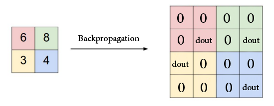
The code we have written for backprop is simply translating this idea to code:

for c in range(C):
      for i in range(H // 2):
        for j in range(W // 2):
          window = x[c, i*2:i*2 + 2, j*2:j*2 + 2]
          max_idx = np.argmax(window)
          max_r = max_idx // window.shape[1]
          max_c = max_idx % window.shape[1]
          dx[c, i*2:i*2+2, j*2:j*2+2][max_r, max_c] += dout[c, i, j]

One thing to keep in mind is that np.argmax() returns an index instead of (row, col) so we have to convert it appropriately, then index into it to incrementally build up dx.

Softmax

To complete our implementation of a CNN, we need a fully connected layer that flattens the tensor we get from the last conv layer (most likely with non-linearity and pooling applied) into a $k$-dimensional vector where $k$ is the number of classes. For our MNIST classifier, we have digits, so $k = 10$.

We also apply a softmax activation to the predictions to convert them into probabilities that add up to 1. To convert these probabilities into a loss we can use for training, we use cross-entropy loss, given by the following formula:

\begin{equation} L=−log(p_c) \end{equation}

where $p_c$ is the probability of the correct class.

As this post is about CNNs, I won’t get into too much detail for softmax / cross-entropy loss. Those who are interested can check out this excellent blog post from Eli Bendersky.

Here are the implementations for a fully-connected linear layer as well as a function computing loss and derivatives for softmax loss.

class Linear:
  def __init__(self, in_features, out_features, weight_scale = 1e-3):
    # Initialise weight matrix of shape (in_features, out_features)
    self.weights = np.random.randn(in_features, out_features) * weight_scale
    self.bias = np.zeros(out_features)

  def forward(self, x):
    """
    Inputs:
    - x: An ndarray containing input data, of shape (d_1, ..., d_k) such that 
      D = d_1 * ... * d_k is equal to `in_features`
    Returns:
    - out: output, of shape (1, out_features)
    """
    self.x_before_flatten = x # cache
    reshaped_x = x.flatten()[np.newaxis, :] # shape (1, D)
    self.x_after_flatten = reshaped_x # cache

    # @ is the matrix multiplication operator in Python
    # reshaped_x's shape: (1 , D)
    # self.weight's shape: (D , M) where M is out_features
    # result of reshaped_x @ self.weights is of shape (1, M), so (1,10) for MNIST
    out = reshaped_x @ self.weights + self.bias 
    return out
  
  def backward(self, dout):
    """
    Inputs:
    - dout: An ndarray of the upstream derivatives, of shape (1, M) where M = out_features
    Returns a tuple of:
    - dx: Gradient w.r.t input x, of shape (d_1, ..., d_k)
    - dw: Gradient w.r.t. weights w, of shape (D, M)
    - db: Gradient w.r.t the biases, of shape (M, )
    """
    dx = (dout @ self.weights.T).reshape(*self.x_before_flatten.shape)
    dw = self.x_after_flatten.T @ dout # (D x 1) * (1 x M)
    db = dout.squeeze() # turns (1, M) to (M, )
    return dx, dw, db

def softmax_loss(scores, y):
  """
  Inputs:
  - scores: ndarray of scores, of shape (N, C) where C is the no. of classes
  - y: ndarray of class labels, of shape (N,) where y[i] is the label for x[i] 
  Returns a tuple of:
  - loss: Scalar value representing the softmax loss
  - dscores: Gradient of loss w.r.t scores, of shape (N, C)
  """
  N = scores.shape[0]

  # for each sample, we shift the scores by the maximum value for numerical stability
  # if you are confused, read the bolded section titled "Practical issues: numerical stability"
  # from this page: https://cs231n.github.io/linear-classify/#softmax-classifier
  shifted_scores = scores - np.amax(scores, axis=1, keepdims=True)

  exp = np.exp(shifted_scores) # shape is (N, C)
  probs = exp / exp.sum(axis=1, keepdims=True) # also (N, C)
  cross_entropy = -1 * np.log( probs[np.arange(N), y] ) # shape is now (N,) -> scalar value per sample
  loss = cross_entropy.mean() 

  # calculate derivatives. See https://eli.thegreenplace.net/2016/the-softmax-function-and-its-derivative/
  dscores = probs.copy()
  dscores[np.arange(N), y] -= 1
  dscores /= N

  return loss, dscores

Putting it together

Once we have the core components, we can put together the classes we’ve written so far to create a CNN model:

conv = Conv(1, 8, 3)  # 28x28x1 -> 26x26x8
pool = MaxPool2x2() # 26x26x8 -> 13x13x8
linear = Linear(13 * 13 * 8, 10)  # 13x13x8 -> 10

def forward(image, y):
  '''
    Completes a forward pass of the CNN
    - image is a numpy ndarray of shape (1 x 28 x 28) representing the greyscale image
    - y is the corresponding digit
  '''
  # transform the image from [0, 255] to [0, 1]
  out = conv.forward((image / 255))
  out = pool.forward(out)
  scores = linear.forward(out)

  loss, dout = softmax_loss(scores, y)

  return scores, loss, dout   

def loss(image, label):
  '''
    Computes loss + completes a backward pass of the whole model
  '''
  grads = {}
  # forward pass
  scores, loss, dout = forward(image, label)

  # Backprop
  dpool, grads['W_linear'], grads['b_linear'] = linear.backward(dout)
  dconv = pool.backward(dpool)
  dx, grads['W_conv'], grads['b_conv'] = conv.backward(dconv)

  return loss, grads


# Challenge yourself: can you try to train the model?

I’ve omitted the training part because I wanted to focus on what each component is doing -— can you come up with the code to train the CNN model below on the MNIST dataset? Challenge yourself!

CNN in Keras

So far we’ve walked you through how to implement a CNN from scratch in Python. Fortunately, we practically never have to write a CNN from scratch nowadays, thanks to high-level libraries like Keras that help abstract all the underlying complexity away from us. To finish off this post, let’s use Keras to implement the same CNN that we’ve implemented above. I adapted this example from the official Keras MNIST CNN example .

from tensorflow import keras
from tensorflow.keras import layers
from tensorflow.keras.utils import to_categorical

# split data
(x_train, y_train), (x_test, y_test) = keras.datasets.mnist.load_data()

# scale images
x_train = x_train.astype("float32") / 255
x_test = x_test.astype("float32") / 255

# Make sure images have shape (28, 28, 1)
x_train = x_train[:,:,:, np.newaxis]
x_test = x_test[:,:,:, np.newaxis]

print("x_train shape:", x_train.shape)
print(x_train.shape[0], "train samples")
print(x_test.shape[0], "test samples")

Downloading data from https://storage.googleapis.com/tensorflow/tf-keras-datasets/mnist.npz
11493376/11490434 [==============================] - 0s 0us/step
11501568/11490434 [==============================] - 0s 0us/step
x_train shape: (60000, 28, 28, 1)
60000 train samples
10000 test samples

A few things worth pointing out in the code above:

First, once we load the MNIST dataset, we scale the images so that each pixel is in the [0,1] range instead of [0,255]. This makes it easier for us to train the CNN.

Next, we add a fourth dimension to the x_train and x_test tensors, which were initially of size N x 28 x 28, where N is the number of images. The last dimension we add represents the number of channels each image has, which is 1 because in MNIST we are working with greyscale images. For RGB, you would set this to 3. Also note that we add the number of channels as the last dimension in the Keras example. This is the standard adopted by Keras and Tensorflow. In our numpy implementation above, we adopted the convention used in PyTorch, the other major framework for machine learning, where the number of channels goes before the width and height of the image (i.e. a single image would be represented by a tensor of shape 1 x 28 x 28 instead of 28 x 28 x 1).

Now our images are ready for training! Now let’s turn out attention to our labels.

By default, y_train and y_test are arrays that contain single integers representing the digit that each image represents. Keras, however, expects each target label to be a 10-dimensional vector. Therefore, we use to_categorical() from keras.utils to obtain an array of one-hot encoded vector. That is to say, if our target is 5, then after calling to_categorical(), we would get the zero-indexed array [0. 0. 0. 0. 0. 1. 0. 0. 0. 0.].

Here’s the code, with some helpful outputs to see what’s going on:

# one-hot encoding label vectors
print("y_train[0] before to_categorical: ", y_train[0])

y_train = to_categorical(y_train, 10)
y_test = to_categorical(y_test, 10)

print("y_train[0] after to_categorical: ", y_train[0])

print("y_train shape:", y_train.shape)

y_train[0] before to_categorical:  5
y_train[0] after to_categorical:  [0. 0. 0. 0. 0. 1. 0. 0. 0. 0.]
y_train shape: (60000, 10)

Once we’ve gotten our data ready for training, we now move onto actually specifying the model that we’ll be using. Again, this is almost the exact same model that we’ve implemented from scratch moments ago (the only difference being the presence of ReLU activation following each Conv2D):

model = keras.Sequential(
    [
        keras.Input(shape=(28,28,1)),
        layers.Conv2D(filters=8, kernel_size=(3, 3), activation="relu"),
        layers.MaxPooling2D(pool_size=(2, 2)),
        layers.Flatten(),
        layers.Dense(10, activation="softmax"),
    ]
)

model.summary()

Model: "sequential"
_________________________________________________________________
 Layer (type)                Output Shape              Param #   
=================================================================
 conv2d (Conv2D)             (None, 26, 26, 8)         80        
                                                                 
 max_pooling2d (MaxPooling2D  (None, 13, 13, 8)        0         
 )                                                               
                                                                 
 flatten (Flatten)           (None, 1352)              0         
                                                                 
 dense (Dense)               (None, 10)                13530     
                                                                 
=================================================================
Total params: 13,610
Trainable params: 13,610
Non-trainable params: 0
_________________________________________________________________

We also use a batch size of 1, which means we do gradient descent using gradients accumulated from just 1 image. We also do this for only 1 epoch. These settings are less than ideal, but to keep the Keras example consistent with our CNN implementation, we stick with it to see what kind of accuracy we can get. The official Keras MNIST CNN example , for example, uses a batch size of 128 for 15 epochs with a deeper CNN model and easily achieves ~99% test accuracy on MNIST. Not bad!

We use the Adam optimizer with the categorical_crossentropy loss that we’ve discussed previously, since we have 10 target classes (which is > 2). Keras also allows us to keep track of various metrics during the course of training, and here we specify that we want Keras to report the accuracy.

Let’s compile the model and train it!

batch_size = 1
epochs = 1

model.compile(loss="categorical_crossentropy", optimizer="adam", metrics=["accuracy"])

model.fit(x_train, y_train, batch_size=batch_size, epochs=epochs, validation_split=0.1)

score = model.evaluate(x_test, y_test, verbose=0)
print("Test loss:", score[0])
print("Test accuracy:", score[1])

54000/54000 [==============================] - 266s 4ms/step - loss: 0.1660 - accuracy: 0.9506 - val_loss: 0.0787 - val_accuracy: 0.9792
<keras.callbacks.History at 0x7fa9d01f72d0>

Test loss: 0.08045849204063416
Test accuracy: 0.9753000140190125

After just 1 epoch of training, we obtain a test accuracy of ~97.5% on the MNIST dataset, which is pretty good.

Conclusion

That’s it! To recap, I walked you through how CNNs can be implemented from scratch in Python using just numpy, and we’ve seen how we can specify and train the same CNN model using Keras to reach a ~97.5% test accuracy on the MNIST dataset. Hopefully, the next time you use Keras or PyTorch or Tensorflow or any other similar libraries, remember that all they’re doing at a high level is abstracting away the theory and code covered in this post (except they’re vectorized / optimised for the GPU and thus often significantly faster).

Bits&Brains